Management Accounting:
Concepts, Techniques & Controversial Issues

James R. Martin

Chapter 11 - Example 11-1

The Cal Company produces pocket size calculators that are sold for $10 per unit. The costs associated with each unit are as follows: 

The company’s tax rate is 40%.

In a recent meeting, the board of directors asked the following questions. How many calculators do we need to produce and sell to accomplish each of the following requirements? 
        1. Break-even. 
        2. Earn net income before taxes of $40,000. 
        3. Earn net income after taxes of $24,000.  
        4. Earn a 20% return on sales before taxes. 
        5. Earn a 12% return on sales after taxes.

To answer these questions, we start by calculating the contribution per unit as follows: 

        Contribution margin per unit = P - V = 10 - (3 + .25 + 2 + .75) = 10 - 6 = 4. 

        Then, the five questions are answered by using the equations from Exhibit 11-1.

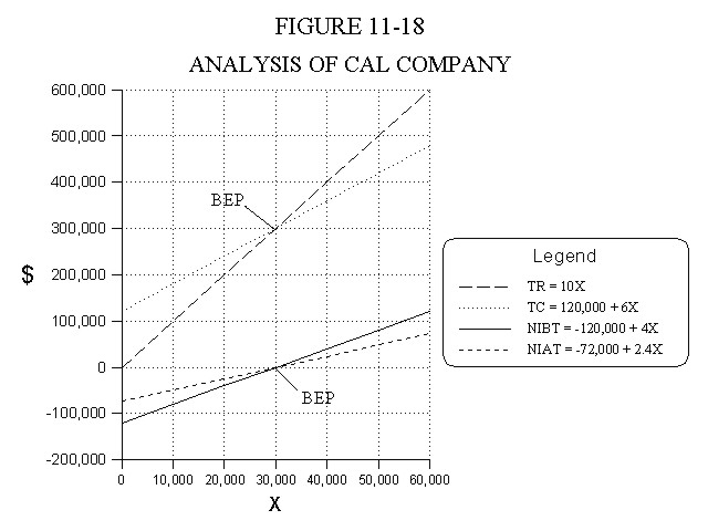
A graphic solution to Example 11-1 is illustrated in Figure 11-18.

Using The After Tax Equations As An Alternative

The equation for NIAT that appears in the graph is found by multiplying the equation for NIBT by (1-T) , i.e., (1-.4)(-120,000 + 4X) = -72,000 + 2.4X. Rearranging this equation we have 2.4X = 72,000 + NIAT. This revised equation indicates that the contribution margin after taxes ($2.4X) is equal to fixed costs after taxes ($72,000) plus the desired after tax income. It provides an alternative way to find the answers to questions 3 and 5 as illustrated below.

3. Earn net income after taxes of $24,000.

   2.4X = 72,000 + NIAT desired
   2.4X = 72,000 + 24,000
   2.4X = 96,000
        X = 96,000 ÷ 2.4 = 40,000 units.

5. Earn a 12% return on sales after taxes.

   2.4X = 72,000 + NIAT desired
   2.4X = 72,000 + .12(10X)
   2.4X = 72,000 + 1.2X
   1.2X = 72,000
        X = 72,000 ÷ 1.2 = 60,000 units.

The accuracy of linear cost-volume-profit calculations can be verified easily. For example, the answers to the questions above can be verified as follows:

1) Is 30,000 units the break-even point? Yes, since total contribution margin is equal to total fixed cost of 120,000, i.e., (4)(30,000) = $120,000. 2) Will 40,000 units generate a before tax profit of $40,000? Yes, because total contribution margin is (4)(40,000) = $160,000 and this amount is 160,000 - 120,000 = $40,000 above total fixed costs. 3) Will 40,000 units generate an after tax profit of $24,000? Yes, since (1-.4)($40,000 NIBT) = $24,000. 4) Will 60,000 units provide a 20% return on sales before taxes? Yes, since the NIBT is TCM - TFC or (4)(60,000) - 120,000 = $120,000. Sales equals PX or ($10)(60,000) = $600,000. R = 120,000 ÷ 600,000 = .20 or 20%. 5) Will 60,000 units provide a 12% return on sales after taxes. Yes, (1-.4)(.2) = .12 or 12%. For an alternative check (1-.4)(120,000) = $72,000 NIAT. Therefore, the after tax rate of return is 72,000 ÷ 600,000 = .12 or 12%.